Introducing MonkQL: the stock-research language your AI agent writes

MonkQL is the language your AI agent writes when you ask Monk.trade a question about the market. Monk.trade is an MCP server, so any agent that speaks MCP can use it. You ask in plain words. The agent writes a few lines of MonkQL, Monk.trade compiles and runs them, and the agent reads back the rows and charts. The query stays short enough for you to check, and a scan of the whole US market comes back in about a tenth of a second.

Why a language, and not SQL or Python? Because the agent writes it and you read it. A query only looks back: close[1] is one bar ago, and there is no way to write tomorrow. Prices, volumes and percentages are types, so comparing a price with a volume fails to compile rather than returning nothing. Loops have fixed bounds, a call has 30 seconds, and nothing runs until the whole query compiles. Filings and financials count from when they became public. A few lines carry all of that.

Every example below is a real session: a question in plain words, the MonkQL the agent wrote, and the result Monk.trade returned. Line breaks are added to fit the page.

A setup is a few lines

We asked for liquid common stocks that broke above their prior 20-day high on at least twice their average volume. The agent wrote:

from stocks on daily
include type == "common"
where sma(close * volume, 20)[1] >= 20000000
  and close > highest(high, 20)[1]
  and volume >= 2 * sma(volume, 20)[1]
show close,
  highest(high, 20)[1] as breakout_level,
  100 * (close / highest(high, 20)[1] - 1) as pct_above,
  volume / sma(volume, 20)[1] as vol_ratio,
  100 * (close / close[1] - 1) as day_chg
sort 100 * (close / highest(high, 20)[1] - 1) desc
take 50

A series like close or volume is the whole history, and [n] reads it n bars back. highest(high, 20)[1] is the highest high of the 20 sessions before today, so today’s bar can break it. sma(close * volume, 20)[1] >= 20000000 keeps stocks that trade at least $20M a day on average; most scans below start with it. The agent then ran the scan on the last completed session and charted the strongest result with the level marked:

Names for the parts

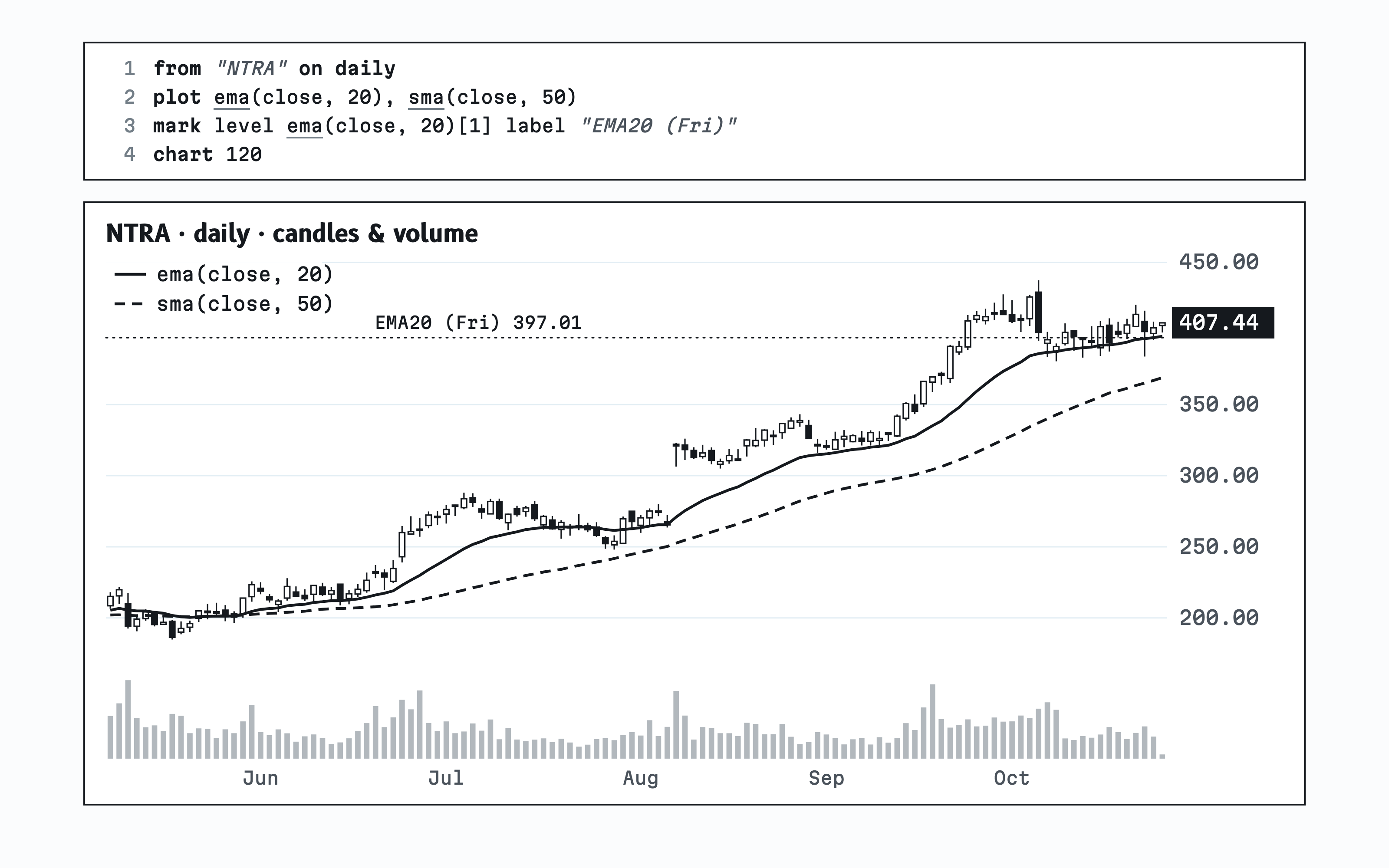
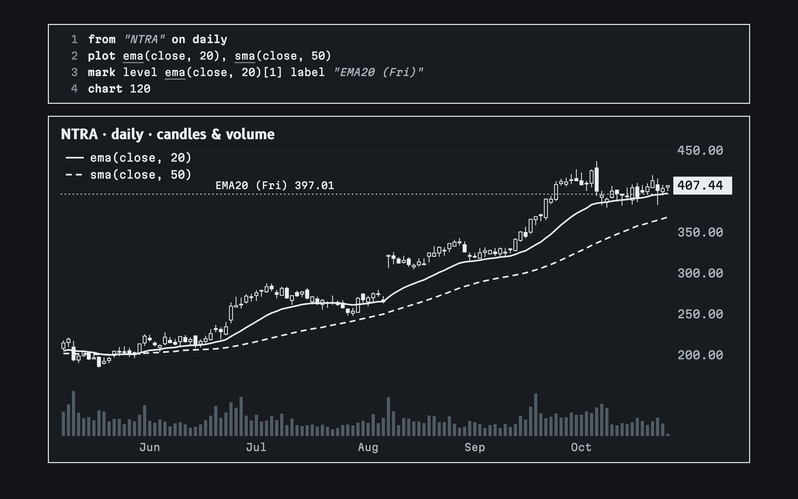
A pullback in an uptrend has more parts, and let names them:

from stocks on daily
include type == "common"
let e20 = ema(close, 20)
let s50 = sma(close, 50)
where sma(close * volume, 20)[1] >= 20000000
  and e20 > s50
  and e20 > e20[5]
  and s50 > s50[5]
  and low <= e20
  and close > e20
  and volume < 0.8 * sma(volume, 20)[1]
show close, e20 as ema20, s50 as sma50,
  100 * (low / e20 - 1) as low_vs_ema_pct,
  volume / sma(volume, 20)[1] as rel_vol,
  count(close > e20, 30) as days_above_ema_30,
  roc(e20, 20) as ema20_roc20
sort count(close > e20, 30) desc
take 25

Each line of where is one rule of the setup: the 20-day EMA above the 50-day average, both higher than a week ago, a low that touched the EMA, a close back above it, and volume under 80% of normal. count(close > e20, 30) counts the sessions out of the last 30 that closed above the EMA, so sorting by it puts the steadiest trends first.

Ranges and levels

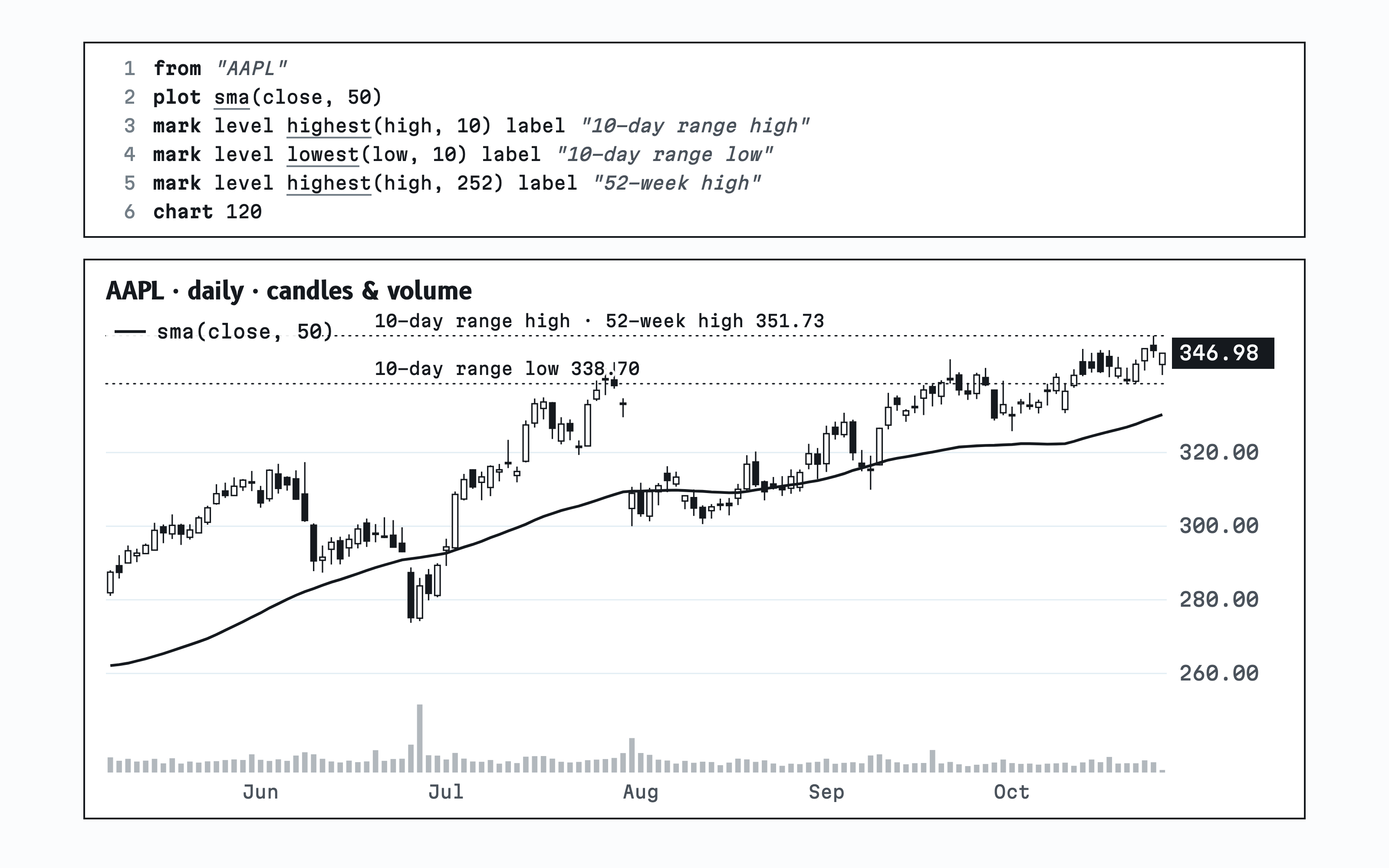
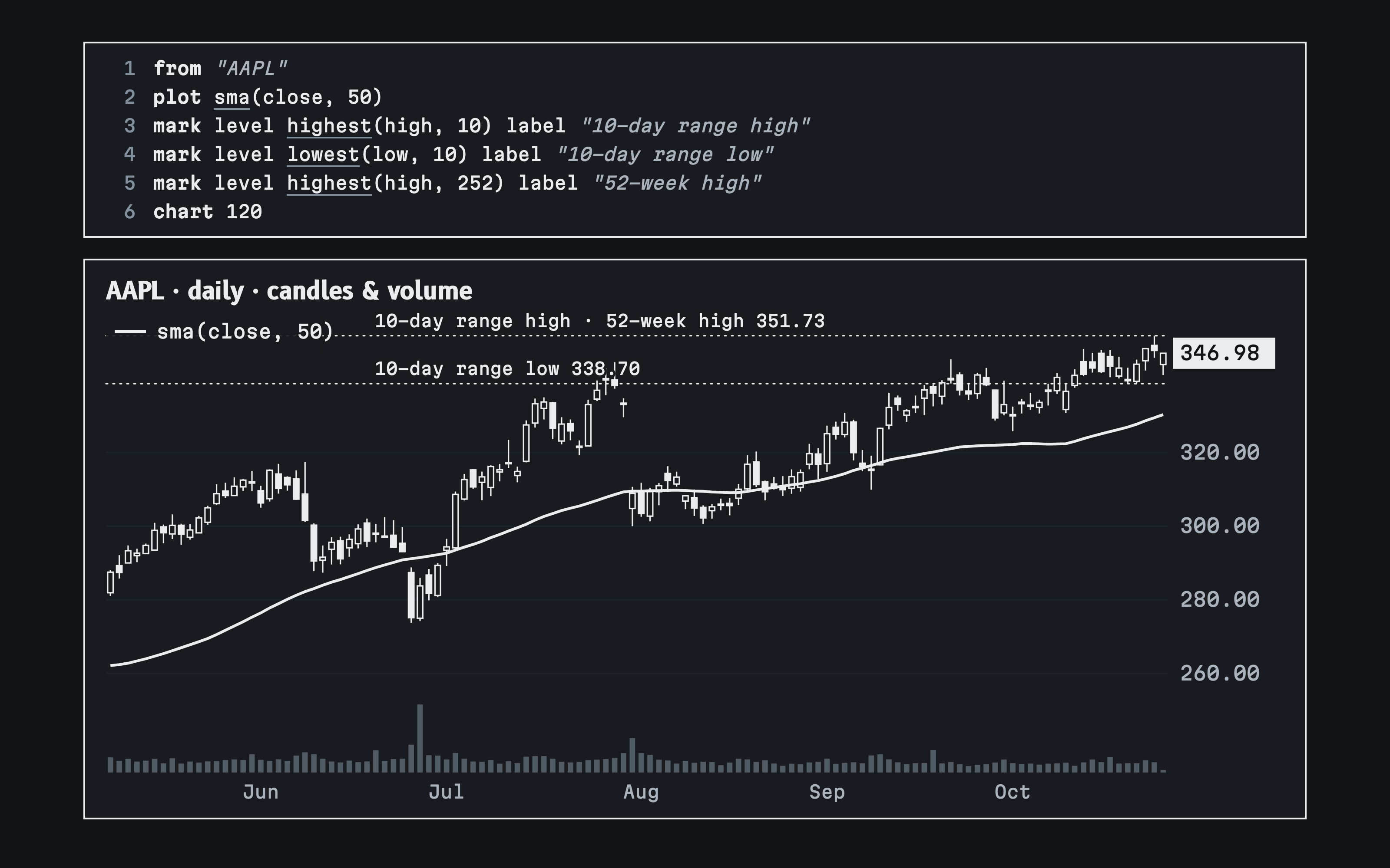
For stocks coiling near their highs, the agent defined the 10-day range as a percentage of price and kept those at their tightest of the last 60 sessions, within 5% of the 52-week high:

from stocks
include type == "common"
let rng = 100 * (highest(high, 10) - lowest(low, 10)) / close
where sma(close * volume, 20)[1] >= 20000000
  and rng <= lowest(rng, 60)
  and close >= 0.95 * highest(high, 252)
show close, rng as range10_pct,
  100 * (close / highest(high, 252) - 1) as from_52w_high_pct,
  sma(close * volume, 20) as dollar_vol20
sort rng asc
take 25

lowest(rng, 60) works on a series the query defined, the same as on close. Charts take expressions too: mark level highest(high, 10) draws whatever the expression evaluates to on the newest bar.

Every timeframe in one call

A line --- separates up to five queries in one call, as in the clip at the top. on picks the interval, and @daily reads the daily series from inside an intraday query, so high@daily[1] is the prior session’s high on a regular-session 5-minute chart.

Extended hours work the same way: on 5m premarket runs on premarket bars, where close@daily is the last regular close. This is how the agent found premarket gaps:

from stocks on 5m premarket
include type == "common"
where 100 * (close / close@daily - 1) >= 3 and volume@premarket >= 10000
show 100 * (close / close@daily - 1) as gap_pct,
  close as pm_last,
  volume@premarket as pm_volume
sort 100 * (close / close@daily - 1) desc
take 100

Across the market

Cross-sectional functions compare each stock with the rest of the scan. Asked for the stock that led each sector over 20 sessions, the agent wrote:

from stocks
include type == "common" and sma(close * volume, 20)[1] >= 20000000
where rank(roc(close, 20) by sector) == 1
show sector, roc(close, 20) as ret20, close,
  sma(close * volume, 20)[1] as dollar_vol
sort roc(close, 20) desc
take 50

Sector	Stock	20-session return
Information Technology	BMBL	+135.4%
Health Care	NAUT	+116.2%
Consumer Discretionary	FIGS	+50.7%
Industrials	OLB	+43.6%
Energy	RRC	+38.8%
Financials	CBOE	+33.6%
Real Estate	CCI	+32.3%
Consumer Staples	LW	+24.7%
Communication Services	TRI	+24.7%
Materials	CLF	+24.6%
Utilities	PNW	+15.8%

include sets the population a rank is taken over and where filters after ranking, so “first in its sector” means first among liquid common stocks, not first among whatever survived other filters. percentile, share, cs_mean and cs_median work the same way. A group smaller than 20 stocks is reported as undecided rather than ranked.

Your own functions

MonkQL has no built-in linear regression. We asked the agent to write one, and it did, in one expression:

fn linreg_slope(x, n) =
  6 * ((n - 1) * sum(i in 0..n - 1 : x[i]) - 2 * sum(i in 0..n - 1 : i * x[i]))
    / (n * (n * n - 1))
let slope = linreg_slope(close, 50)
on daily
include type == "common" and close >= 5 and sma(close * volume, 20)[1] >= 20000000
where slope > 0 and count(crossover(slope, 0), 5) >= 1 and close > sma(close, 200)
show close, slope as slope_per_day,
  100 * slope / close as slope_pct_per_day unit percent,
  since(crossover(slope, 0), 5) as turned_bars_ago,
  100 * (close / sma(close, 200) - 1) as above_200d unit percent,
  sma(close * volume, 20) as dollar_vol_20d
sort sma(close * volume, 20) desc
take 50

fn defines a function, and sum(i in 0..n - 1 : …) is a bounded loop over bar offsets. This is the least-squares slope in closed form. A function can only call functions defined before it, so nothing runs away.

The library grows slowly on purpose. We hold out 48 published daily scans for testing, and a new built-in has to be needed by at least two of them. Linear regression is needed by one, so you write it yourself.

The compiler is the guardrail

Agents know the function names other tools use, so the likely mistake is borrowing one. The compiler turns it into a correction before any data is read:

• Spelling is forgiving: case, a ta. or math. prefix and underscores are ignored, so TA.SMA is sma and cross_over is crossover.
• Vocabulary is not. MA and HHV are errors whose hints name sma and highest, because a name from another tool can carry that tool’s meaning. The only synonyms are avg and mean for sma, sum of a condition for count, and if(c, a, b) for c ? a : b.
• Expressions carry units. Prices, volumes, ratios and percentages are different types, so close > volume is “cannot compare price with volume”, not an empty result.
• [n] only counts back. A written negative offset is a compile error, because it would read the future.
• The parser recovers at the next clause and the checker keeps going, so one compile reports every problem it can find. The query in the clip returned all three of its problems at once, each with a hint.

Every query that compiles comes back in a canonical form, with keywords and names in lower case, one clause per line, numbers in one notation and defaults such as from universe all, on daily and take 100 written out. Queries that differ only in case, spacing, clause order, synonyms or omitted defaults print the same text and share a digest. The result carries that text, so you can see exactly what ran.

Fast enough to ask again

An agent works by asking, reading and asking again, so every query has to come back before the conversation moves on. Ranking every sector across all 13,270 US-listed symbols took 129 milliseconds of server time; the breakout scan took 133 and the regression scan 173. Each result also reports what it set aside and could not decide, so the agent can say what it left out.

Server time per call, across all 13,270 US-listed symbols

Leader of every sector

129 ms

Breakout on volume

133 ms

50-day regression slope

173 ms

Median, a week of calls

130 ms

How it runs

The compiler is Rust: a lexer, a recursive-descent parser, a checker for names, types and units, and a planner. The plan is a deduplicated expression graph, so sma(close, 20) used in where, show and a chart mark is computed once per stock, with the warm-up history recursive functions like ema need. Evaluation runs per stock over column buffers, and a node is computed on first demand, so a stock that fails the first where condition computes nothing else.

The language is about 41,000 lines of Rust with 560 tests, among them generative tests that compile random programs, valid and broken, and print the seed of any failure.

Beyond stocks and price

The same language runs on 34 futures contracts with from futures, and saved queries keep a version history you can rerun. The same expressions also read SEC filings, Form 4 insider trades, reported financials and news as series aligned with the bars, each counted from when it was published or filed, never from the date it describes. That is a post of its own.

Try it

Connect Monk.trade to your agent with the guides for Claude, ChatGPT or other MCP apps, then ask for a setup in plain words. The quickstart and the full MonkQL reference are served to the agent with the tools, and the agent will show you every query it runs.

• A call holds at most five queries in 8,192 bytes and has 30 seconds.
• Market-wide scans start from active US stocks (premarket and after-hours scans skip that floor); ETFs and other types stay in unless the query filters them, as these examples do with type == "common".
• Queries are read-only.